/8 min read/Audio & acoustics/AI / ML/Scientific computing/audio · ai · pytorch · cuda · dsp · optimization
Fitting a bell with four thousand guesses
The capstone: a differentiable copy of the modal bar, a loss that had to be taught to hear decay, and a GPU running thousands of random initializations in parallel until one of them finds the physics.
Part 3 of 3Plucked, Struck, BlownAll parts →Part 1 built a bar out of nine damped resonators with decay times we verified to three significant figures. That exactness was the point: the bar is a synthesizer whose true parameters we know. So here’s the inverse problem, with an answer key. Hand a recording of the bar to an optimizer that has never seen the Faust source, just a bank of damped sinusoids,
and ask gradient descent to find the modes. If it can pass the exam where we
know the answers, we’re allowed to point it at recordings where we don’t.
Everything below ran on the RTX 5090 in
the project repo;
fit/fit_modal.py is ~250 lines of PyTorch.
Why this needs four thousand guesses
The sine-plus-cosine trick makes amplitude and phase linear, the easy part. The decays are tame too. The frequencies are the trap. A spectral loss, as a function of , is a comb of narrow valleys: move a candidate mode 3% off a true partial and the gradient toward it vanishes into noise floor. There is no smooth path from “mode at 700 Hz” to “mode at 1213 Hz”; a candidate is either born near a partial or it never finds one.
The classical answer is clever initialization. The GPU answer is to be clever and run four thousand initializations anyway, because a batch of independent fits is embarrassingly parallel: every candidate synthesizes its waveform, takes its STFTs, and steps its own Adam state in lockstep, as one big tensor op. Stage A runs waves of 1024 random candidates (log-uniform frequencies, one candidate seeded from FFT peak-picking) on a short crop; the best 64 survivors refine on a long window in stage B.
The loss I wrote first, and what it refused to hear
The standard recipe is multiscale spectral loss: compare magnitudes at several window sizes, L1, linear plus log. My first version worked beautifully — for the wrong definition of beautifully. High modes came back to ±0.01 cents. And the fundamental’s ten-second decay came back as 0.9 seconds. The forgery had perfect pitch and no sustain, like a bell struck through a pillow.
The autopsy was embarrassing in the way good bugs are. The loss averaged over every cell of every spectrogram, hundreds of thousands of them. The fundamental’s dying tail lives in maybe ninety frames of one frequency bin; its total contribution to the mean was about . The optimizer traded the entire tail for a microscopic improvement to the attack, because the attack is loud and the mean is a democracy of cells. Meanwhile the same loss recovered 14 kHz modes to a hundredth of a cent, because up there, a cent is several bins wide and visible. A magnitude loss hears exactly what its resolution lets it hear, no more, and it will happily spend your tail to polish your transient.
Two changes made decay non-negotiable. The log-magnitude term went to full weight, since faint modes live there. And I added a log-RMS envelope term: the signal’s loudness contour at about 20 Hz frame rate, weight 2. The envelope has only a few hundred frames, so a wrong tail can’t hide in its mean. This is the actual lesson of differentiable DSP, in my experience of one long night: the model was never the hard part; the loss is where you tell the truth.
The exam, graded
Four thousand and ninety-six candidates (four waves of 1024), each with 14 modes, 500 Adam steps on a ¾-second crop: stage A takes 297 seconds at about 6,900 candidate-steps per second. Every step synthesizes a waveform, takes three STFTs and an envelope, and backpropagates through all of it. The 64 survivors then refine on eight seconds for 1500 steps (168 s). Whole exam: under eight minutes of GPU time.
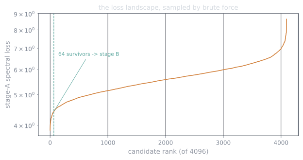
The landscape justifies the brute force. Stage-A losses ran from 3.86 (best) to 8.65 (worst): a 2.2× spread on the same data from initialization luck alone. A single clever start is a lottery ticket; four thousand is a census. (My FFT peak-picking “smart” candidate, which aced the earlier magnitude-only loss, didn’t even make the top 64 under the envelope-aware one. Priors are humbling.)
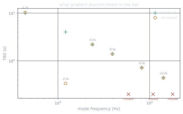
Recovered against the answer key, six of nine modes, four essentially exact:
| designed | recovered | pitch error | designed t60 | recovered |
|---|---|---|---|---|
| 440.00 Hz | 439.57 Hz | −1.7 c | 10.00 s | 10.28 s |
| 1212.86 Hz | 1210.8 + 1224.2 Hz | split† | 4.01 s | 0.34 + 4.55 s |
| 2377.72 Hz | 2377.26 Hz | −0.33 c | 2.19 s | 2.21 s |
| 3930.52 Hz | 3930.49 Hz | −0.01 c | 1.39 s | 1.39 s |
| 8200.68 Hz | 8200.62 Hz | −0.01 c | 0.72 s | 0.72 s |
| 14138.39 Hz | 14138.58 Hz | +0.02 c | 0.44 s | 0.44 s |
† the fit spent two components here, a fast one for the strike transient plus a 4.55 s ring 16 cents high. A legal decomposition, just not the bookkeeping I asked for. The test that matters is behavioral: measure the decay of the resynthesized forgery the same way we measured the target, and the instrument comes back: 10.28 / 4.18 / 2.21 s against the target’s measured 10.02 / 4.02 / 2.19 s.
Notice the pattern in the pitch errors: ±0.01 cents above 4 kHz, a few cents below 1 kHz. That’s not mysticism, it’s bin width. At 440 Hz a cent is a hundredth of an STFT bin; at 14 kHz it’s most of one. A magnitude loss resolves frequency exactly as well as its windows do, and no better.
Three modes never came back: 5871, 10919, and 17834 Hz, the faintest in the recording (the strike position sits near their node lines, and they die in under a second). Sixty-four survivor slots went to candidates that spent their modes where the loss lived instead. Brute force finds what’s loud; what’s faint still takes luck we didn’t buy tonight.
The string, forged by a bell
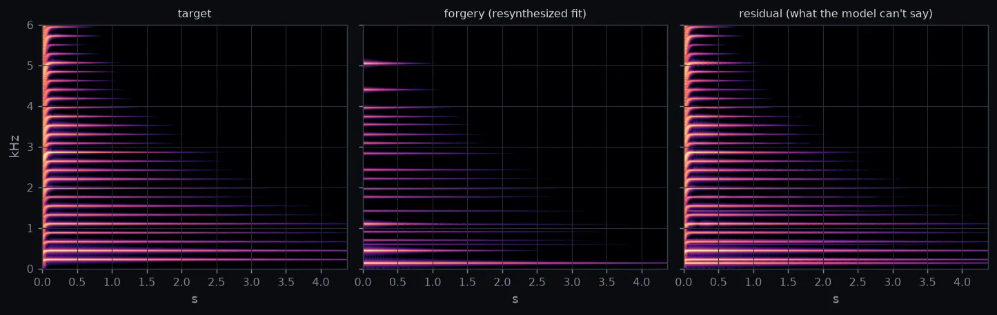
The first attempt was a rout. The bar has nine well-separated modes; random frequencies land near them often enough that a census finds every loud one. A plucked string is the opposite terrain: forty partials spaced exactly 220 Hz apart. Here 4096 random candidates produced confident garbage, components at 673 and 1141 Hz, between the rungs, nothing on the fundamental. Density, not sparsity, is what breaks random search; there are too many valleys and they’re all narrow.
The half-fix costs one line: seed a single candidate per wave with the harmonic ladder , leaving every frequency free to move (the fit should measure the string, not be told about it). With the seed, the mid and upper ladder snaps into lock: partials 15, 17, 18, 20, and 31 land within 2 cents, partial 2 within 1, and the fit reads off the loop filter’s damping law directly from audio. Measured on the forgery versus the target, band by band:
| partial | target t60 | forgery t60 |
|---|---|---|
| 6813.9 Hz | 0.48 s | 0.48 s |
| 5046.0 Hz | 0.81 s | 0.84 s |
| 3958.2 Hz | 1.20 s | 1.28 s |
| 1096.2 Hz | 4.02 s | 1.44 s |
| 440.1 Hz | 4.81 s | 1.91 s |
The treble half of the instrument, frequency and decay, is essentially perfect. The bass half got shortchanged, and the reason is visible in the budget: 24 free modes against 40 real partials means something starves, and under a spectral loss the money goes where energy is densest, which for this pluck was the crowded top of the comb. The exam grades itself: a bank of free modes is the right tool for a bell and a spendthrift way to describe a string.
Which points at the real sequel. Part 1 knows this instrument: its partials are one fundamental, a stretch law, and a damping law. Three functions, not seventy-two free parameters. Swap the mode bank for that structured model and the whole comb costs less than the bell did. The difference between curve-fitting and physics-fitting is exactly the difference between 24 modes and 3 laws, and it’s where this series goes next if it goes anywhere.
What the residual knows
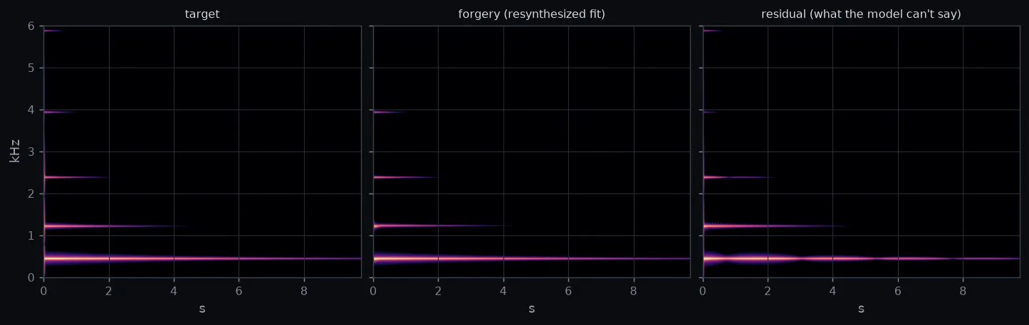
Subtract the forgery from the target and you hear what the model has no words for. For the bar, the residual is almost entirely the first few milliseconds: the mallet’s noise, the one thing a damped sine can’t be. For the string it’s that plus the unpaid debt, every partial the mode budget skipped. The residual is the honest boundary of your model as a theory of the sound, rendered as audio you can play.
The scripts take any WAV. The obvious next targets are not synthesizers at all: a wine glass, a radiator, a stairwell handrail. Strike, record, fit, and read off the modes of an object that never had a datasheet.