/4 min read/Quantum/Scientific computing/quantum · gpu · cuquantum · tensor-networks
A hundred qubits in four milliseconds (terms and conditions apply)
cuTensorNet stops storing the state and the qubit ceiling evaporates; the wall comes back wearing a different coat. Measured to the knee, plus what the whole series adds up to.
Part 5 of 5One GPU, N QubitsAll parts →Four parts of this series treated one assumption as physics: to simulate qubits you store amplitudes. Parts 1–4 measured that assumption’s price: a hard budget of 30-ish qubits, then a cliff.
But the assumption is a choice. If what you want from a circuit is one number (an amplitude, an expectation value, a correlator) you don’t need the whole state at any point. A quantum circuit is a network of small tensors (one per gate) glued along shared indices, and the amplitude is what falls out when you contract the entire network down to a scalar. Storage stops scaling with qubit count; it scales with the largest intermediate tensor the contraction order produces. That’s what cuTensorNet does, and its Python API is disarmingly small:
from cuquantum import tensornet as tn
conv = tn.CircuitToEinsum(circuit, dtype="complex128", backend=cp)expr, operands = conv.amplitude("0" * n)      # an einsum, not a statevectornet = tn.Network(expr, *operands)path, info = net.contract_path()              # cost model runs BEFORE you payamp = net.contract()
That info object is the underrated hero: it tells you the estimated FLOPs
and the largest intermediate before you commit, which makes “should I
even attempt this” a question you can answer in milliseconds. All numbers
below are from
bench/05_tensornet.py.
Width is free
GHZ states: maximally entangled in the textbook sense, but with a simple, tree-like circuit structure. Amplitude of , which should be exactly :
| Qubits | Contraction | Amplitude returned |
|---|---|---|
| 32 | 10.0 ms | 0.707107 |
| 64 | 2.8 ms | 0.707107 |
| 100 | 4.1 ms | 0.707107 |
A 100-qubit amplitude in four milliseconds, correct to six digits. For scale: the statevector for 100 qubits would need bytes, about , a hundred million times all the storage humanity has ever manufactured. The contraction never materializes it, so it never pays for it. Qubit count, the villain of parts 1–4, has simply left the story.
Depth is not
Something else must pay instead, and a second circuit family finds it: brickwork random circuits, alternating layers of random single-qubit rotations and CX bricks, the standard stand-in for “genuinely entangling, no exploitable structure.” Width fixed at 32 qubits, depth cranked:
| Depth | Est. FLOPs | Largest intermediate | Contraction |
|---|---|---|---|
| 8 | 1.1×10⁵ | tiny | 43 ms |
| 16 | 4.7×10⁷ | tiny | 14 ms |
| 20 | 1.4×10⁹ | 8 MiB | 85 ms |
| 24 | 1.8×10¹¹ | 4 GiB | 569 ms |
| 28 | 1.8×10¹¹ | 2 GiB | 1,068 ms |
| 32 | 2.7×10¹³ | 8 GiB | over budget |
| 40 | 5.4×10¹³ | 8 GiB | over budget |
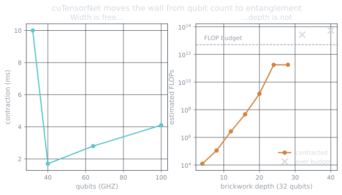
The estimated cost climbs nine orders of magnitude while the qubit count never moves. Around depth 24 the intermediates hit gigabytes and a single amplitude costs half a second; by depth 32 the optimizer quotes FLOPs and my benchmark’s self-imposed budget (5×10¹², roughly “a few seconds of GPU”) declines to pay. The wall from part 1 is back. It just changed currency, from bytes of state to entanglement the contraction has to squeeze through. Physicists will recognize the shape: for volume-law circuits, treewidth grows with depth×width, and the exponential always collects eventually.
One more honest ledger line: the path-finding isn’t free either. It cost 1.5 s of CPU hyper-optimization at depth 40, before any GPU work. And a single amplitude is not a simulation: sampling bitstrings from a deep random circuit needs many amplitudes or smarter (and costlier) contraction strategies. Width-versus-depth is a genuine trade, not a loophole.
What one GPU actually buys: the series ledger
Every number measured on one RTX 5090 (driver 610.62, CUDA 13 runtime wheels, cuQuantum 26.6.0, cuPy 14.1.1, Qiskit 2.5.0, WSL2 Ubuntu 24.04), reproducible from the repo:
| Regime | Ceiling | Speed |
|---|---|---|
| Statevector, fp64 | 30 qubits | ~1.45 TiB/s effective (87% of the card’s memory bandwidth) |
| Statevector, fp32 | 31 qubits | same bandwidth, half the bytes, one more qubit |
| Driver sysmem spill | +1–2 qubits | 7× to 72× per-gate penalty; emergencies only |
| Managed memory (WSL2) | worse than the spill in every measured way | 34 GiB/s, flat |
| Tensor network, structured/shallow | 100+ qubits | milliseconds per amplitude |
| Tensor network, volume-law | depth ~28 at width 32 | ~1 s per amplitude, exponential past it |
The one-sentence version: a consumer GPU simulates quantum circuits at the speed of its memory and the size of its memory. Every route past that trades exponentially in some other direction. Which is, of course, the whole reason quantum hardware is worth building.
Where this series goes next, when bench time allows: cuQuantum 26.6 shipped two new libraries, cuStabilizer (Clifford circuits at scales where none of this article’s math applies) and cuPauliProp, and error correction is where those shine. A logical qubit needs a few thousand physical gates per cycle; simulating that pipeline on this card is a different series, and the itch has already started.