/7 min read/Audio & acoustics/audio · dsp · faust · physical-modeling
Three instruments in sixty lines each
A plucked wire, a struck bar, and a blown pipe, built from physics instead of samples. Including the afternoon the pipe refused to play the note I asked for, and the measurement that explained a famous magic constant.
Part 1 of 3Plucked, Struck, BlownAll parts →There are two ways to make a computer sound like an instrument. You can record an instrument and play the recording back; that’s sampling, respectable and solved. Or you can teach the computer the physics and let the sound fall out. The second way is called physical modeling, and its dirty secret is how little code it takes: each instrument in this series is about sixty lines of Faust, and every timbral knob corresponds to something you could point at on the real object. Pick position. Mallet hardness. Blowing pressure.
I built three, one per way of making an object vibrate: a plucked wire, a struck bar, a blown pipe. They live in this repo, they play in your browser (part 2), six pieces performed on them hang in the sound gallery, and in part 3 I make a GPU listen to one and reverse-engineer it. Everything below is measured, not asserted; the measurement scripts are committed next to the instruments.
Better than reading about them: play them. The workbench below is the actual instruments, compiled to nine kilobytes of WebAssembly each (part 2 explains how), running live in your tab once you press power.
The playable workbench needs JavaScript. Without it, the pieces in the gallery are the same instruments, recorded.
The wire: Karplus–Strong, taken seriously
The 1983 Karplus–Strong algorithm is the “hello world” of physical modeling: fill a delay line with noise, loop it through a mild lowpass, and out comes a shockingly convincing plucked string. The reason it works is that it is a string (the delay line is the wave’s round trip, the filter is energy loss), so the way to make it better is to take the physics more seriously, term by term.
My version adds four things, each one a real property of a real string:
- Pick hardness. The excitation is one period of noise through a lowpass at Hz. A thumb and a plectrum differ mostly in how much treble they let into the string.
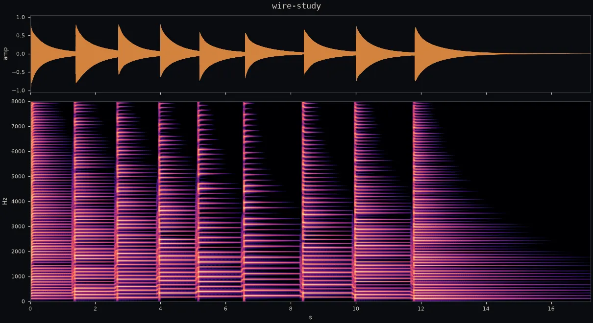
- Pick position. Plucking at fraction of the length notches every harmonic with a node there: a feedforward comb, . In the gallery piece Wire study you can watch the notches walk as the pluck point moves toward the bridge.
- Decay as a physical parameter. The loop multiplies by once per round trip, and a round trip happens times a second, so gives exactly a -second decay to −60 dB. No magic gain constants: you ask for a five-second string, you get one.
- Dispersion. Real steel is stiff, and stiffness makes high frequencies travel faster, which stretches upper partials sharp. That is the piano’s signature inharmonicity. Three first-order allpasses with a negative coefficient reproduce it: group delay falls with frequency, upper partials see a shorter string, and they land sharp on cue.
The delay line then makes up whatever the filters didn’t use, so the loop still totals one period. Measured against intent: a 220 Hz pluck comes out at 219.93 Hz, 0.6 cents flat. I’ll take it.
The bar: nine modes and a contact time
A struck metal bar doesn’t have harmonics. A free–free bar (xylophone key, glockenspiel plate) vibrates at measured ratios of the fundamental,
and that refusal to line up is why metal sounds like metal. So the bar model doesn’t simulate a waveguide at all. It’s modal synthesis: nine resonant filters at those ratios, each rung by the same strike and left to ring with its own decay time, , high modes dying faster the way damping in real materials prefers.
Two parameters carry all the musical character, and both are geometry:
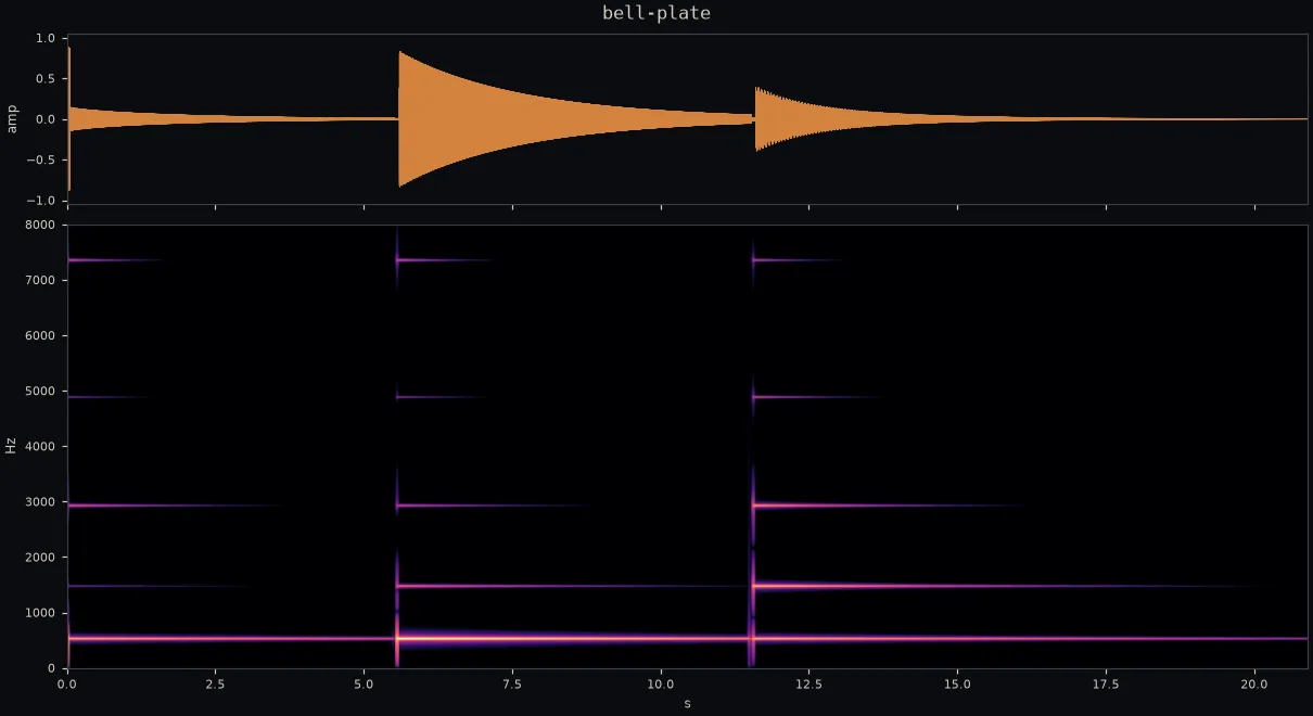
- Strike position weights each mode by whether you hit its node line: , so a center strike mutes the even modes and an edge strike wakes everything. The gallery piece Bell plate is one bar struck three ways; the chord changes because the node-line arithmetic does.
- Strike hardness is a contact time, not a volume. The strike is a raised-cosine force pulse between 0.2 ms (hard mallet) and 3.2 ms (soft), and a pulse that long simply can’t push on a mode whose period is shorter than the contact. That is the physically honest lowpass. Soft mallets don’t “filter” the bar; they never excite it.
Because every mode is an explicit filter with an explicit decay, this instrument is checkable, and I checked it. Designed versus measured, from the calibration strike at 440 Hz:
| mode | designed | measured |
|---|---|---|
| 440.0 Hz | 10.00 s | 10.02 s |
| 1212.9 Hz | 4.02 s | 4.02 s |
| 2377.7 Hz | 2.20 s | 2.19 s |
Mode frequencies land within a quarter cent. This exactness is the setup for part 3: if the synth is a sum of decaying sines with known parameters, a fit that claims to recover them can be graded against an answer key.
The pipe: the loop picks its own note
The blown pipe is a different animal, because unlike the wire and the bar it is an oscillator: energy goes in continuously, and the pitch is whatever frequency the feedback loop decides to sing at. You don’t set the note. You negotiate.
The model is Cook’s slide-flute topology from STK: breath pressure feeds a jet delay into a cubic nonlinearity , which dumps into a bore delay closed by an inverting lowpass reflection, the open pipe end. The cubic is the whole flute. Below it’s just an inverting gain, and the loop hisses quietly; push the pressure past the fold and the waveform creases once per round trip, and that crease is the tone. Blow harder still and it chokes. My model speaks from breath ≈ 0.95 and gives up past ≈ 1.35, which anyone who has played a recorder will recognize as fair.
Then I asked it for 440 Hz and got 607.
Naively, a bore one period long should resonate at the period. Instead the measured pitch sat a wide, consistent interval sharp, so instead of re-deriving jet-drive theory at 3 a.m. I did the empirical thing: a grid over bore lengths and jet ratios, measuring what came out. One line of the grid was rock solid. With the jet at a third of the bore, every bore length (in target periods) produced
four bore lengths agreeing to the third decimal. Which means the loop is an inverting resonator speaking on its m = 1 odd mode at . The flute is always overblown. Set the bore periods long and the note lands on pitch.
And here’s the part I enjoyed most: STK’s Flute::setFrequency multiplies
the requested frequency by a bare, uncommented 0.66666 before computing
its delay. . That constant is this measurement,
fossilized. Cook knew; the code just never said.
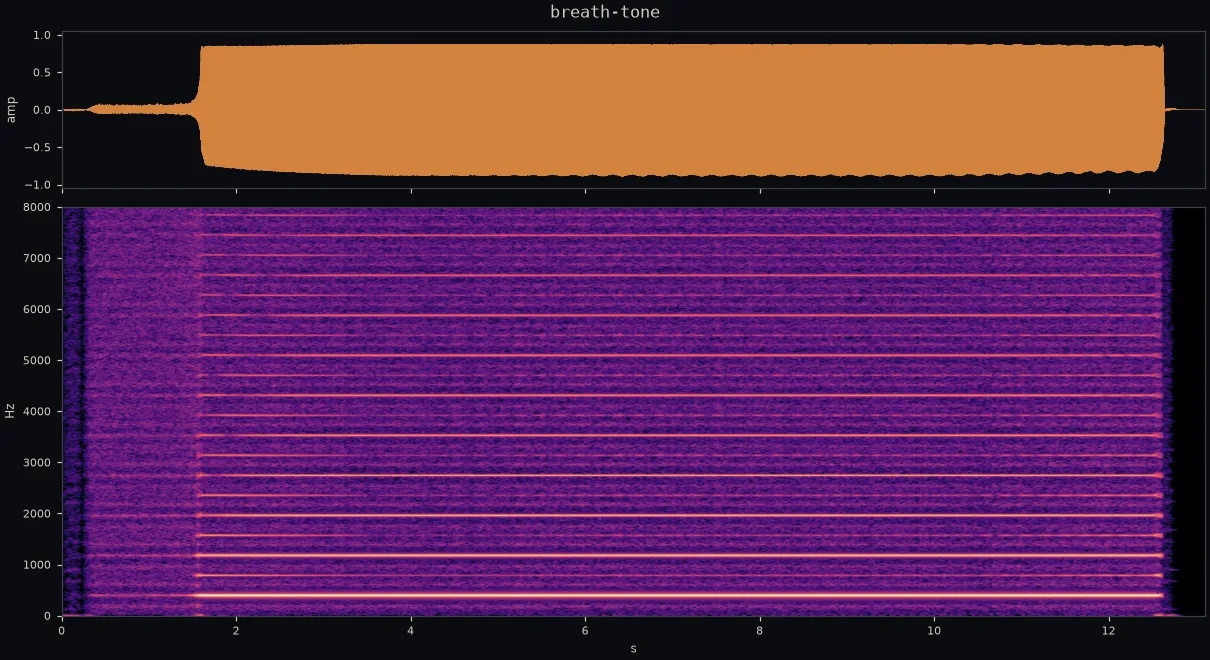
Calibrated, the pipe holds its register from C4 to G6 within 6 cents (below C4 it jumps registers, which is what short pipes do; the slider now stops where the physics does). Vibrato is applied to breath, not frequency, because that’s where flutists put it. Articulation in the gallery piece Air phrase is nothing but a 60 ms dip below speaking pressure.
One lesson the hard way
The gamelan piece wants a low gong ringing under a melodic run played on the same bar. First render: the moment the run retuned the instrument, the gong’s tail bent with it, because a ringing resonator’s state lives inside its filter coefficients, and you cannot move the poles without moving the sound already inside them. The fix is the same one every polyphonic synth ever shipped: another voice. The renderer now runs one modal bank per voice and sums them, and the gong rings out unbothered for eighteen seconds.
Next: compiling all three to WebAssembly small enough to embed in a blog post, and rendering the gallery pieces from Node. The entire wire, physics and all, is nine kilobytes.